1. Draw the dependencies
A Bayesian network represents a joint probability distribution with a directed acyclic graph. Nodes are random variables; the graph and conditional probability tables together define how the joint distribution factorizes.
Use two binary variables: Rain and Grass, with an edge from Rain to Grass. The model says P(Rain, Grass) = P(Rain) × P(Grass | Rain). It is an intentionally simplified example, not a weather forecasting model.
2. Specify probabilities
State order matters: Rain is ["Rain", "No rain"], and Grass is ["Wet", "Dry"]. The rain prior is [0.3, 0.7]. Grass's first row is [0.9, 0.1] given rain; its second is [0.1, 0.9] given no rain. Every row sums to one.
These are supplied assumptions, not parameters learned from data. Wet grass is still possible without rain, which keeps observing grass from identifying rain with certainty. Add all edges before setting tables. With multiple parents, verify the implementation's parent ordering before flattening a table.
3. Query the prior and posterior
Install CoolBox with the matching setup guide. Python's binding takes a two-dimensional CPT and returns one query-state probability with infer. The native C++ implementation accepts flattened tables and returns a full state distribution with query. They are different interfaces to the same example distribution; do not swap their table formats or method names.
from ml_toolbox import bayesian_network

network = bayesian_network.BayesianNetwork()
rain = network.add_node("Rain", ["Rain", "No rain"])
grass = network.add_node("Grass", ["Wet", "Dry"])
network.add_edge(rain, grass)

# Rows are parent states; columns are this node's states.
network.set_cpt(rain, [[0.3, 0.7]])
network.set_cpt(grass, [[0.9, 0.1], [0.1, 0.9]])

prior = network.infer(rain, 0, {})
wet = network.infer(grass, 0, {})
posterior = network.infer(rain, 0, {grass: 0})
dry_posterior = network.infer(rain, 0, {grass: 1})
assert abs(wet - 0.34) < 1e-9
assert abs(posterior - 0.27 / 0.34) < 1e-9
print(f"P(rain): {prior:.6f}")
print(f"P(wet): {wet:.6f}")
print(f"P(rain | wet): {posterior:.6f}")
print(f"P(rain | dry): {dry_posterior:.6f}")
The binding's matrix converter accepts these rectangular nested sequences. Its Python package manages its declared dependencies; no plotting package is needed.
No working discrete Bayesian-network API was found in the current Go binding for this walkthrough. Use the Python or native C++ example rather than assuming the boosted-tree or finance bindings imply Bayesian-network support. Check the current Go source for updates.
The current Rust BayesianNetwork is a placeholder: methods such as add_node and set_cpt return unsupported-operation errors. A type name alone is not functional inference support. Use Python or C++, and check the Rust implementation before using it.
#include <cmath>
#include <exception>
#include <iomanip>
#include <iostream>
#include <stdexcept>
#include <bayesian_network.h>

int main() {
    try {
        BayesianNetwork network;
        const int rain = network.add_node("Rain", {"Rain", "No rain"});
        const int grass = network.add_node("Grass", {"Wet", "Dry"});
        network.add_edge(rain, grass);
        network.set_cpt(rain, {0.3, 0.7});
        network.set_cpt(grass, {0.9, 0.1, 0.1, 0.9});
        const auto prior = network.query(rain);
        const auto wet = network.query(grass);
        const auto posterior = network.query(rain, {{grass, 0}});
        const auto dry_posterior = network.query(rain, {{grass, 1}});
        if (std::abs(wet[0] - 0.34) > 1e-9
            || std::abs(posterior[0] - 0.27 / 0.34) > 1e-9) {
            throw std::runtime_error("Inference check failed");
        }
        std::cout << std::fixed << std::setprecision(6)
                  << "P(rain): " << prior[0]
                  << "\nP(wet): " << wet[0]
                  << "\nP(rain | wet): " << posterior[0]
                  << "\nP(rain | dry): " << dry_posterior[0] << '\n';
        return 0;
    } catch (const std::exception& error) {
        std::cerr << error.what() << '\n';
        return 1;
    }
}
Use C++17 and the bayesian_network_ai/headers include directory, or link the installed CoolBox::bayesian_network CMake target. CoolBox contains other headers named bayesian_network.h; this example specifically uses the native discrete, variable-elimination implementation, not the separate Python-wrapper header.
4. See the update
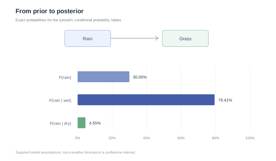
The marginal probability of wet grass is 0.3 × 0.9 + 0.7 × 0.1 = 0.34. Bayes' rule gives P(rain | wet) = 0.27 / 0.34 ≈ 0.794118. Observing dry grass instead gives 0.03 / 0.66 ≈ 0.045455.
Do not reverse conditionals: P(wet | rain) = 0.9 is not P(rain | wet). The rain prior and alternative explanations matter. Conditioning on an observation is also not the same as intervening on a variable; these arrows alone do not establish causal effects.
5. Extend carefully
Add a sprinkler parent to Grass to model another explanation, then provide a row for every parent-state combination. Keep all entries finite, between zero and one, and each row normalized. Avoid impossible evidence: conditioning on an event with zero model probability has no defined posterior.
Exact inference can become expensive as a network grows. Start with small graphs, validate manually computable queries, and consult the native discrete-network API before assuming support for parameter learning, continuous variables, or approximate inference.