This is an educational numerical example, not investment advice. Black-Scholes assumes European exercise, no dividends in these formulas, constant volatility and interest rates, and frictionless trading. Its output is not a prediction of investment returns.
1. Set up the finance API
Use the Python, Go, Rust, or C++ setup guide. These examples target a current CoolBox checkout with the finance bindings; an older compiled extension may not expose them.
Python uses finance.evaluate, Go uses EvaluateFinanceFormula, and Rust uses evaluate_finance_formula. Each accepts a formula selector and numeric inputs. C++ exposes named functions in finance.hpp; link the installed CoolBox::FINANCE CMake target.
2. Define one option contract
For the Black-Scholes formulas used below, input order is spot, strike, risk-free rate, volatility, maturity in years. Set spot and strike to 100, the continuously compounded annual rate to 0.05, annualized volatility to 0.20, and maturity to 1 year. Rates are fractions, not percentages: 0.20 means 20%.
A call pays max(S − K, 0) at expiry; a put pays max(K − S, 0). Pricing today discounts the model's risk-neutral expected payoff. The prices below use the same currency units as spot and strike.
3. Price, measure, and compare
Each tab is a complete program: calculate call and put prices, check put-call parity, read call delta and vega, and reprice the call at three volatility levels. No NumPy, Matplotlib, or separate finance package is needed for these formulas.
from math import exp
from ml_toolbox import finance

F = finance.Formula
spot, strike, rate, volatility, years = 100.0, 100.0, 0.05, 0.20, 1.0
inputs = [spot, strike, rate, volatility, years]
call = finance.evaluate(F.BLACK_SCHOLES_CALL_PRICE, inputs)
put = finance.evaluate(F.BLACK_SCHOLES_PUT_PRICE, inputs)
delta = finance.evaluate(F.BLACK_SCHOLES_CALL_DELTA, inputs)
vega = finance.evaluate(F.BLACK_SCHOLES_VEGA, inputs)
residual = (call - put) - (spot - strike * exp(-rate * years))
assert abs(residual) < 1e-9, "Put-call parity failed"

print(f"Call: {call:.6f}; put: {put:.6f}")
print(f"Call delta: {delta:.6f}")
print(f"Vega per 1 percentage point: {vega * 0.01:.6f}")
for sigma in [0.10, 0.20, 0.40]:
    price = finance.evaluate(
        F.BLACK_SCHOLES_CALL_PRICE, [spot, strike, rate, sigma, years]
    )
print(f"Volatility {sigma:.0%}: call {price:.6f}")package main
import (
"fmt"
"log"
"math"
coolbox "github.com/MeanderingAI/CoolBox/_deliverables/libraries/bindings/go_bindings"
)
func main() {
spot, strike, rate, volatility, years := 100.0, 100.0, 0.05, 0.20, 1.0
evaluate := func(formula coolbox.FinanceFormula, sigma float64) float64 {
value, err := coolbox.EvaluateFinanceFormula(
formula, spot, strike, rate, sigma, years,
)
if err != nil { log.Fatal(err) }
return value
}
call := evaluate(coolbox.BlackScholesCallPrice, volatility)
put := evaluate(coolbox.BlackScholesPutPrice, volatility)
delta := evaluate(coolbox.BlackScholesCallDelta, volatility)
vega := evaluate(coolbox.BlackScholesVega, volatility)
residual := (call - put) - (spot - strike * math.Exp(-rate * years))
if math.Abs(residual) >= 1e-9 { log.Fatal("Put-call parity failed") }
fmt.Printf("Call: %.6f; put: %.6f\n", call, put)
fmt.Printf("Call delta: %.6f\n", delta)
fmt.Printf("Vega per 1 percentage point: %.6f\n", vega * 0.01)
for _, sigma := range []float64{0.10, 0.20, 0.40} {
fmt.Printf("Volatility %.0f%%: call %.6f\n",
sigma * 100, evaluate(coolbox.BlackScholesCallPrice, sigma))
}
}use coolbox_rs::{evaluate_finance_formula, FinanceFormula as F};
fn main() -> Result<(), String> {
let (spot, strike, rate, volatility, years): (f64, f64, f64, f64, f64) =
(100.0, 100.0, 0.05, 0.20, 1.0);
let inputs = [spot, strike, rate, volatility, years];
let call = evaluate_finance_formula(F::BlackScholesCallPrice, &inputs)?;
let put = evaluate_finance_formula(F::BlackScholesPutPrice, &inputs)?;
let delta = evaluate_finance_formula(F::BlackScholesCallDelta, &inputs)?;
let vega = evaluate_finance_formula(F::BlackScholesVega, &inputs)?;
let residual = (call - put) - (spot - strike * (-rate * years).exp());
if residual.abs() >= 1e-9 {
return Err("Put-call parity failed".to_string());
}
println!("Call: {call:.6}; put: {put:.6}");
println!("Call delta: {delta:.6}");
println!("Vega per 1 percentage point: {:.6}", vega * 0.01);
for sigma in [0.10, 0.20, 0.40] {
let price = evaluate_finance_formula(
F::BlackScholesCallPrice, &[spot, strike, rate, sigma, years],
)?;
println!("Volatility {:.0}%: call {price:.6}", sigma * 100.0);
}
Ok(())
}#include <cmath>
#include <exception>
#include <iomanip>
#include <iostream>
#include <stdexcept>
#include <finance.hpp>
int main() {
try {
const double spot = 100, strike = 100, rate = 0.05;
const double volatility = 0.20, years = 1;
const auto call = finance::black_scholes_call_price(
spot, strike, rate, volatility, years);
const auto put = finance::black_scholes_put_price(
spot, strike, rate, volatility, years);
const auto delta = finance::black_scholes_call_delta(
spot, strike, rate, volatility, years);
const auto vega = finance::black_scholes_vega(
spot, strike, rate, volatility, years);
const auto residual = (call - put)
- (spot - strike * std::exp(-rate * years));
if (std::abs(residual) >= 1e-9) {
throw std::runtime_error("Put-call parity failed");
}
std::cout << std::fixed << std::setprecision(6)
<< "Call: " << call << "; put: " << put
<< "\nCall delta: " << delta
<< "\nVega per 1 percentage point: " << vega * 0.01 << '\n';
for (const double sigma : {0.10, 0.20, 0.40}) {
std::cout << "Volatility " << sigma * 100 << "%: call "
<< finance::black_scholes_call_price(
spot, strike, rate, sigma, years) << '\n';
}
return 0;
} catch (const std::exception& error) {
std::cerr << error.what() << '\n';
return 1;
}
}4. Interpret the results
Rounded to six decimals, the call is 10.450584, the put is 5.573526, and call delta is 0.636831. Put-call parity checks C − P = S − K exp(−rT); the residual should be close to zero, allowing for floating-point rounding.
Delta is the local change in option price for a one-unit spot move. It is a sensitivity, not a forecast or a guaranteed hedge. Native vega is per unit of volatility (1.0); multiplying by 0.01 gives approximately 0.375240 per one-percentage-point change. This is a local approximation, not the exact repricing for a large move.
The volatility sweep produces call prices of approximately 6.804958 at 10%, 10.450584 at 20%, and 18.022951 at 40%. Hold all other inputs fixed when interpreting that comparison. Higher volatility raises the value of this vanilla option; that is not a general claim about every derivative.
5. Plot Monte Carlo confidence bands
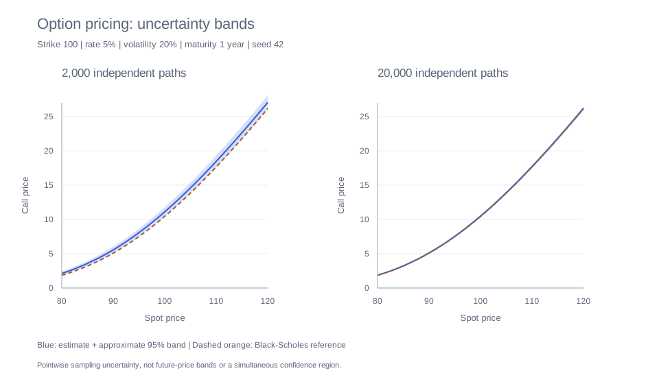
Download the complete native simulation and SVG exporter. Build it like the earlier C++ example, link CoolBox::FINANCE, and pass an output SVG filename when running it. No extra plotting library is needed. The exporter reprices spots from 80 to 120 with strike 100, rate 5%, volatility 20%, and one year to maturity.
For a European terminal payoff, a single one-year geometric-Brownian step is sufficient here. The first 2,000 shocks are a subset of the 20,000-path sample. Each panel reuses its shocks across spots to make comparisons less noisy, so neighboring estimates are correlated; the bands are pointwise, not a simultaneous confidence region.
The package also exposes geometric Brownian paths, digital and barrier formulas, Asian options, and Monte Carlo estimates with standard errors and confidence intervals. Start with the European call above as a closed-form reference before exploring more complex contracts.
Monte Carlo APIs accept time-step durations and standard-normal shock paths, not cumulative dates or already-scaled Brownian increments. Use the risk-free rate as the drift for risk-neutral pricing under this model, fix a seed for reproducible experiments, and increase independent path counts to study sampling error. A simulation confidence interval describes estimator uncertainty, not a range of future market prices.
Check the native finance API and the Python finance bindings for each contract's exact argument order. Barrier and digital formulas do not all take the same input vector as a vanilla option.